5.2. More fun with Gnuplot¶

Let’s use gnuplot to plot some more mathematical functions. Certainly we’ll need more than just polynomials in x as we used on the last page.

Gnuplot has many builtin math function which you can plot. Try the following plot.

If gnuplot is running on your computer, end it by typing quit at the prompt. Then start it again by typing gnuplot. This is just to clear out the previous settings, and to show you how to get out when you are done.

Now that it’s running again, type:

gnuplot> plot exp(-x**2/20) * sin(x)

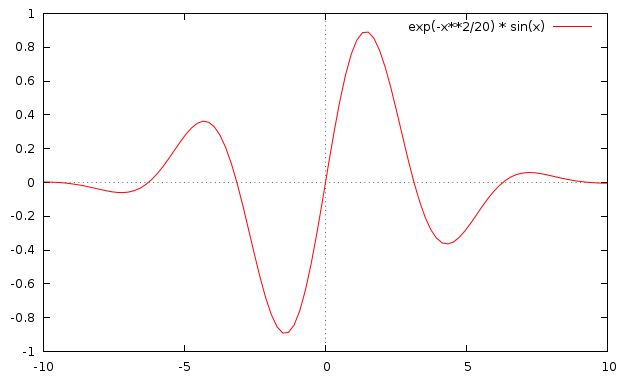
You may want to turn on the zero axis (remember how?). Later we’ll learn how to set that as the default behavior at startup. The plot you just made is of the function

where you used the common exp() and sin() functions. A complete list of functions is here:

Gnuplot Builtin Math Functions

Please have a look at these.

For example, gnuplot will plot the two lowest Bessel functions, J0(x) and J1(x). From these two, the higher order Bessel functions can be constructed. Bessel functions are used in the solution of certain differential equations, particularly in cylindrical coordinates, and turn up often in the physics of musical instruments.

Gnuplot also knows about imaginary numbers and certain constants like $\pi$ .

Try this:

Start gnuplot, then type the following:

gnuplot> print pi
gnuplot> w = 5.8
gnuplot> v = 3.0
gnuplot> print w/v
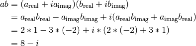
gnuplot> a = {2.0, 3.0}
gnuplot> b = {1.0, -2.0}

In the first line, you asked gnuplot to print the value of ” pi”.

You can also use pi as a value in a range limit, as in plot [-pi:pi].

In the last two lines you defined two variables, a and b , as complex numbers. The first number in the bracket is the real part and the second of course, is the imaginary part.

What is the product ab ? You should remember from junior high:

$ab &= ( a_{\rm real} + i a_{\rm imag} )( b_{\rm real} + i b_{\rm imag} ) \\ &= a_{\rm real} b_{\rm real} - a_{\rm imag} b_{\rm imag} + i (a_{\rm real} b_{\rm imag} + a_{\rm imag} b_{\rm real} ) \\ &= 2*1 - 3*(-2) + i*(2*(-2) + 3*1) \\ &= 8 - i$

Now in gnuplot, do:

print a*b

Does gnuplot confirm your complex arithmetic?

Here $i = \sqrt{-1}$ .

Note

For some incomprehensible reason, engineers tend to use the letter j for the square root of -1. While this is completely ridiculous, I point it out so that you will be aware of the pitfall. Physicists tend to use i. If you are a bit rusty on complex numbers and how to manipulate them, here are a couple links to brush up.

5.2.1. A Simple Calculator¶

Since gnuplot has many builtin math functions, will store things in variables, and will do calculations and print the result, you can use it as a simple scientific calculator. Often, when I’m working on my computer and don’t want to grab my calculator (which I actually don’t enjoy using that much), I just fire up gnuplot and do a little calculation there. Here’s an example: Suppose I want to compute the following quantity

when r = 2.5 and R = 3.9

You could simply start gnuplot and enter the following ( Please perform the steps below:

gnuplot> r = 2.5
gnuplot> R = 3.9
gnuplot> result = 4*pi**2 * r**2/sqrt(R**2 - r**2)
gnuplot> print result
82.4300852943585
gnuplot>

Much easier! . Really.

Try it–have your mom type in the above while you compute the same thing on your caculator.

I bet your mom wins.

5.2.2. Solving Equations Graphically¶

If it’s not already running, start gnuplot.

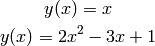
Plot the two equations you used on the previous webpage, [Step One: Build in Math Functions]

$y(x) = x y(x) = 2x^2 -3x + 1$

Set the x range to [-0.5:2] [Step Two: Plot Range.]

Turn on the zeroaxis [also in section: Step Two: Plot Range].

Notice that $2x^2 - 3x + 1$ factors into $2(x - 0.5)(x - 1)$ .

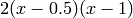Note

Verify this if you don’t see it immediately (i.e. write out the second expression and show that it’s equal to the first).

Thus the exression $2x^2 - 3x + 1$ has roots at $x = 0.5$ and $x = 1$ . Remember, a root is the x value, $x_{\rm root}$ , where the $y(x_{\rm root}) = 0$

Is this corroborated by your plot? In other words, you can see on your plot the places where the equation 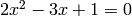$2x^2 - 3x + 1 = 0$ is satisfied, and do you get the values: 0.5 and 1.0.

Now let’s do something a little more interesting.

The x values where the line intersects the parabola are given by the solutions to the equation:

$y(x)_{\rm parabola} &= y(x)_{\rm line} 2x^2 - 3x + 1 &= x$

This equation is slightly more non-trivial to solve; you have to use (OMG!) The Quadratic Formula, and the solutions are

$x = \pm \frac{\sqrt{2}}{2}$

Note

Verify this.

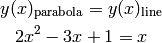
Numerically , these solutions are at x = 0.29289 and x = 1.70711,

Does this look correct from your graph?

You can get a rough anwser by using the mouse. As you move the mouse cursor around in the plot area, notice that the x, y values of where the mouse cursor is, are printed in the bottom left corner of the gnuplot window.

This can give you a pretty good idea of the value of something in your graph.

Here’s another method to solve the equation above, instead of the quadratic formula.

We can zoom in and find where exactly the intersection lies. If you successively narrow the plot range, you can “zero in” in the intersection point. Do the following (use the UP arrow to recall each previous line):

gnuplot> plot [1.5:2] x, 2*x**2 - 3*x + 1
gnuplot> plot [1.7:1.71] x, 2*x**2 - 3*x + 1
gnuplot> plot [1.706:1.708] x, 2*x**2 - 3*x + 1
gnuplot> plot [1.707:1.7072] x, 2*x**2 - 3*x + 1
gnuplot> plot [1.7071:1.70712] x, 2*x**2 - 3*x + 1

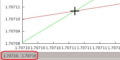
Notice how the successive narrowing of the x range allows us to find the x value of the intersection of the two equations (represented with red and green plots) by reading it from the x axis.

Try the same thing by narrowing the x range around the other root near x = 0.293

This probably seems pretty simple, and not very useful since we already know the solution of the above equation from the quadratic formula.

What about a situation where you don’t know the solution of the equation by analytic (like the quadratic formula) methods? In this case the only way to get the result is to use numerical methods, whihc means that we use a computer to find an approximate (and hopefully very accurate) solution.

5.2. More fun with Gnuplot¶

5.2.1. A Simple Calculator¶

5.2.2. Solving Equations Graphically¶

Table Of Contents

Previous topic

Next topic

This Page