6.6. A Worked Example: Theory meets Experiment¶

In Homework 2 you visited Johnny Utah, a BASE jumping video, photography, and stunt company who have data collected from a long freefall. You should all have a file with this data.

I decided to check out how good this data is.

Also, the distance data is in feet and speed data in miles/hour . It would be easier to convert this to meters and m/s . We can do this by taking advantage of the using feature when plotting data.

To find how to convert, I will use the Unix units program, a wonderful little text based program that gives you conversion factors for one set of units to MANY others.

In an xterm, you should be able to type ” units” at the prompt and get:

sci[~]|>units

2438 units, 71 prefixes, 32 nonlinear units

You have: feet
You want: meters
        * 0.3048
        / 3.2808399
You have: mph
You want: m/s
       * 0.44704
        / 2.2369363

Now, I can set two conversion factor constants in gnuplot that I will use later.

gnuplot> f2m = 0.3048
gnuplot> mph2mps = 0.44704

6.6.1. Theoretical Expectations from Physics¶

You probably know that for an object in free fall in the Earth’s atmosphere, it begins to drop as if there is no air resistance, so the distance from the starting point increases as

$y(t) = \frac{1}{2}gt^2$

where g = 9.8 m/s 2 .

At first, before the object is moving very fast, this will be a good approximation. So let’s check it.

Here’s your data from Homework 4.

Ok. Here’s the data file:

 22   16    16
 42   46    62
 61   76    138
 72   104   242
 87   124   366
 96   138   504
 103  148   652
 107  156   808
 111  163   971
114  167   1138
117  171   1309
119  174   1483
119  174   1657
119  174   1831
119  174   2005
119  174   2179
119  174   2353
119  174   2527
119  174   2701
119  174   2875

Plot it.

gnuplot>plot "MYfreefall.dat" u 1:(f2m*$3), 0.5 * 9.8 * x**2

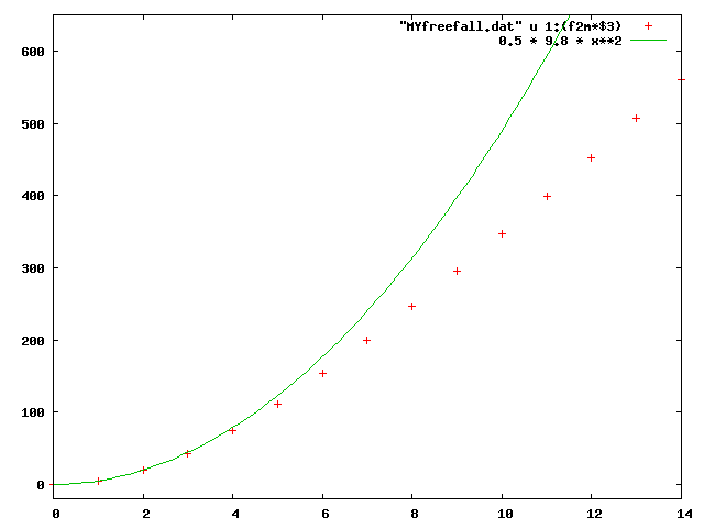
At the beginning of the graph (for small t ), does the function match the data? Do you understand how I converted it to meters by simply using the using command and the constant f2m? Make sure you do.

Fairly quickly, the force of air resistance becomes apparent and once the force of gravity and the force of air resistance are equal, the object will no longer accelerate (right?

$F_{\rm gravity} - F_{\rm air} = 0$

So,

$F_{\rm total} = 0$

With no net force on the falling object, it will no longer accelerate, since $F = ma$ , for those who haven’t had Physics in a while).

If the acceleration is zero, it’s speed will be constant. This speed is called terminal velocity. We can see that on our plot, after about 8 seconds–the position increases linearly (i.e. like a line).

Looking at your data file, the position data in column 3 seems to make sense: quadratic ( $\sim t^2$ ) at the beginnig, and linear (:math:`sim t) at the end, as expected. We’ll deal with the velocity data later.

We can estimate the terminal velocity by plotting a line along with the data and varying its slope until we get it to match the linear part of the data, after 8 sec. It helps to offset the line with a negative b constant ( a*x - b ).

Try to estimate the terminal velocity by plotting the data, AND a line a*x + b. Vary the constant a and b until the line goes though (as best you can) the points from t >= 10.

Now for the theory.

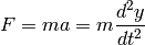
The governing equation here is Newton’s: $F = ma$

We all know that one, right? However, What it really means is this.

where F is the total force $F_{\rm gravity} - F_{\rm air}$ , m is the mass, and the acceleration, a, is the second derivative of position x(t) with respect to time.

$F = ma = m\frac{d^2 y}{dt^2}$

I am being pedantic here for those who have not had calculus for some time. I will shortly get to differential equations–if you have not had DiffEQs , don’t worry–this is just an example. Nonetheless, follow as much as you can.

Recall that the force on a falling object due to gravity is constant

$F_{\rm gravity} = mg$

Now, it turns out that except for rather slow speeds, the force of air resistance can be approximated by a force which grows as the square of velocity

$F_{\rm air} = -kv^2$

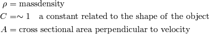
The constant k depends on a number of things

$k = \frac{1}{2}\rho CA$

where:

$\rho &= {\rm mass density} \\ C &= \sim 1 ~~~{\rm a~constant~related~to~the~shape~of~the~object} \\ A &= {\rm cross~sectional~area~perpendicular~to~velocity}$

Let’s simplify the differential equation:

$F = ma$

or

$ma &= F \\ m\frac{d^2y}{dt^2} &= mg - kv^2 \\ \frac{d^2y}{dt^2} &= g - \frac{k}{m}\left(\frac{dy}{dt}\right)^2\\ \frac{d^2y}{dt^2} + \frac{k}{m}\left(\frac{dy}{dt}\right)^2 - g &= 0 \\ \frac{d^2y}{dt^2} + b\left(\frac{dy}{dt}\right)^2 - g &= 0$

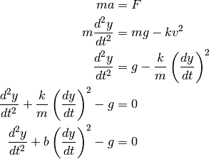
In the last differential equation, we have defined $b = k/m$ . This is the one we have to solve for the function y(t) .

I will skip the solution of this equation (it is done in many books on Differential Equations, as well as many jr. level Physics texts. There is a good review that I found:Auburn Engineering Course).

The function $y(t)$ is

$y(t) = \frac{1}{b}\log\left[\cosh(\sqrt{bg}~t)\right]$

where g is the acceleration of gravity, and b = k/m is as defined above. cosh() is the hyperbolic cosine.

See if you can check that this equation $y(t)$ satisfies the differential equation in the last line above!

6.6.2. Theory meets Experiment¶

If you visit the webpage above to look at the method of solution, or even if you just verify that the solution satisfies the DiffEQ, you can see that this was a non-trivial result. How well does it match the experimental data?

All we have to do to check is to fit the solution to the data. Remember that gnuplot (almost) always uses x for the horizontal axis even though we are calling it t in our theoretical discussion. Similarly, we have called the position x(t) even though it’s been plotted on the y axis. ...Just wanted to be clear.

gnuplot>f(x) = 1/b*log(cosh(sqrt(b*g)*x))
gnuplot> fit f(x) "MYfreefall.dat" u 1:(f2m*$3) via g, b
...
Final set of parameters            Asymptotic Standard Error
=======================            ==========================

g               = 10.0539          +/- 0.0284       (0.2824%)
b               = 0.00338874       +/- 2.414e-05    (0.7123%)
...

gnuplot>plot "MYfreefall.dat" u 1:(f2m*$3), f(x)

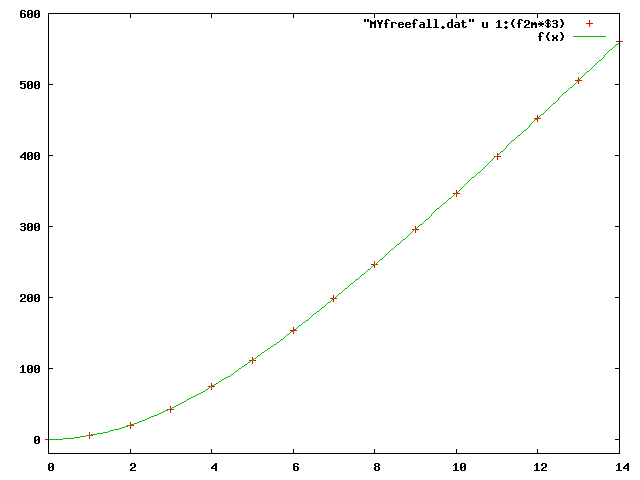
BANG!

The theoretical function is really good fit to the data. Also the fitted value for g is rather close to the known value (9.8):

gnuplot> print (g-9.8)/9.8 * 100
2.59118938657317

within about 2.6%. Notice that in the fit report above, the error on the value for g is 0.284 = 2.8%. Thus the data is consistent with the known value of g=9.8 m/s.

That’s not too bad for pulling some data from an extreme sports webpage and applying the laws of physics!

6.6.3. Velocity¶

Next lets look at the velocity. Given the position, $y(t)$ , the velocity is just the time derivative:

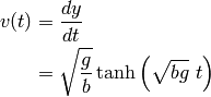
$v(t) &= \frac{dy}{dt} \\ &= \sqrt{\frac{g}{b}}\tanh\left(\sqrt{bg}~t\right)$

Check this. You may have to consult your math book to recall the derivative of cosh(x) .

Now we can check the velocity data against the data. Recall that the velocity data is in the stupid units: mph = miles per hour . However, our constant mph2mps takes care of that. So, define the function v(x) , and plot the data and theory.

gnuplot>v(x) = sqrt(g/b)*sinh(sqrt(b*g)*x)/cosh(sqrt(b*g)*x)
gnuplot>plot "MYfreefall.dat" u 1:(mph2mps*$2), v(x)

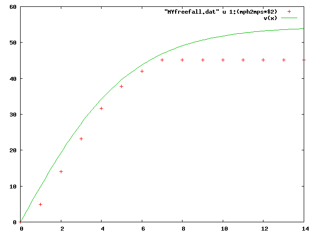
The match between theory and experiment is not good.

The key thing to realize here is that velocities are usually measured by taking the initial and final positions over some time interval $\Delta t$ , then dividing the change in position $\Delta y$ by $\Delta t$ to get the average speed over that interval. Thus the velocity really represents the speed closer to the middle of the time interval. The velocity recorded at, say, 3 seconds, really should be reported as the speed at 2.5 seconds , since the last measurement of position was made at 2 seconds. Does this make sense to you? In other words, the velocity data should really be shifted back (left) by 0.5 second in time. That’s easy to do with using!

gnuplot>plot [0:20] "MYfreefall.dat" u ($1-0.5):(mph2mps*$2), v(x)

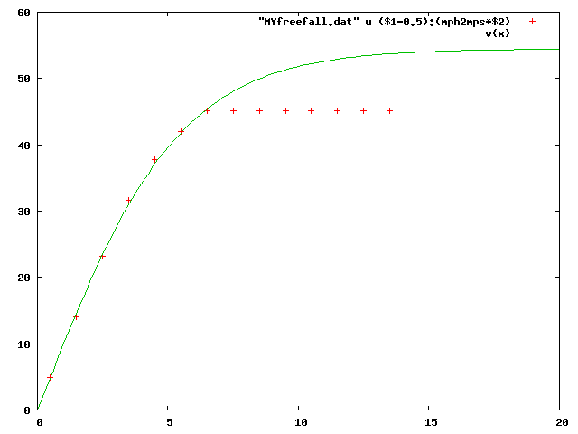
Much better.

I also added an extended plot range to the graph so we could see the approach to terminal velocity, and how long it takes to get to a constant speed.

We also see that the ” Terminal Speed” reported in the original data is not quite correct.

The falling object has not yet obtained constant speed. You might want to plot thus using a ” using ” trick like:

gnuplot> u 1:($1>7 ? $2 : 1.0/0)

which will block plotting any points after 7 seconds. Do you see how it works?

6.6.4. Forensic Data Analysis¶

When you think of forensics, you probably think of CSI of a crime show. Forensic data analysis, is about reconstructing what you can about something from the data you have.

Let’s see if we can figure out the mass of the jumper!

From our fit, we know that b, the coefficient of air resistance, is

b = 0.0033

Hence, we can estimate the parameters in this equation. The density of air, $\rho$ , is about 1 kg/m 3. The “Shape Coefficient”, C , for a prone falling human is around 1 (it’s probably slightly higher but to our level of accuracy, 1 will do; see the article on Drag Coefficients at Wikipedia).

The surface of a falling person is also hard to estimate, but let’s say a 6 foot person (~1.8 m) times a width of half a meter. That’s $0.9 m^2$ .

That means that the mass of our falling person is about

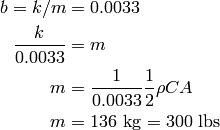
$b = k/m &= 0.0033 \\ \frac{k}{0.0033} &= m \\ m &= \frac{1}{0.0033}\frac{1}{2} \rho C A \\ m & = 136~{\rm kg} = 300~{\rm lbs}$

That seems a bit high, but it could easily be

a 220 lb man*, with a 50 lb parachute + reserve chute + 30 lbs of

camera and position/speed measuring gear. or + a 180 lb instructor + 100 lb student + 20 lb of gear

3: :///home/jhetrick/www/phys27/pages/gnuplot/solnHW3.html .. _Auburn Engineering Course: http://www.eng.auburn.edu/department/me/courses/nmadsen/egr182a/drag01.html .. _Wikipedia: http://en.wikipedia.org/wiki/Drag_coefficient#Cd_in_other_shapes .. _Vertical Visions: http://www.vertical-visions.com/ .. _Homework 2: :///home/jhetrick/www/phys27/pages/gnuplot/../editor/hw2.html

6.6. A Worked Example: Theory meets Experiment¶

6.6.1. Theoretical Expectations from Physics¶

6.6.2. Theory meets Experiment¶

6.6.3. Velocity¶

6.6.4. Forensic Data Analysis¶

Table Of Contents

Previous topic

Next topic

This Page