11.2. Linear Algebra
There is another commercial package for doing math which is very popular, particularly among engineers, that you should know about: MATLAB
Matlab stands for “Matrix Laboratory”, which gives you some indication of its purpose. Linear Algebra is the mathematics of matrices and vectors, but that’s almost the simplest way to think about it. It’s the mathematics of systems of linear equations (which can be written in matrix form, no matter how many, and many other related topics.
In fact, we will be not be using Matlab, but rather a free “clone” with much of Matlab‘s functionality, called Octave. More on that below.
Back to Linear Algebra.
Believe me, linear algebra is a FREEKING DEEP subject. It should be required of all physics and engineering students, and included in PACS. Almost everything you have learned in advanced math has a linear algebra connection.
This is very useful for many things:
- Many data sets can be thought of as a long vector. Calculations on these data can be done by MATLAB. An example might be Stock Market data over some period of time.
- Systems of linear equations. Many other problems, such as partial differential equations, statics problems, fluid dynamics, etc. can be given a matrix/linear algebra form. See: Finite Element Methods
- Many things, like the set of all periodic functions
 can be represented
as a set of vectors in an infinite dimensional vector space. That’s
Fourier Analysis...
can be represented
as a set of vectors in an infinite dimensional vector space. That’s
Fourier Analysis... - Signal Processing. MATLAB has many tools for signal analysis, Fourier transforms, audio and image processing (after all an image is just a matrix of pixel values–see what I mean about most problems having a linear algebra representation?).
- Representing rotations, tranlations (both from one language to another as well as the physics meaning: movement from place to another in space. Actually, if you think about Heisenberg’s Matrix Formulation of Quantum Mechanics, in fact Change in general can be represented by an infinite dimensional matrix in the space of all possibilities...
- Representing symmetry.
...just to name a few.
We are fortunately going to take baby steps into linear algebra.
Whereas Mathematica was a tool whose primary use is for symbolic (algebraic) calculations, MATLAB is fundamentally numerical. That means that it manipulates matrices and vectors as tables and arrays of numbers (like [1, -1, 3]), not as algebraic symbols (like a, b, g, and x ) as Mathematica did.
11.2.1. Matrix Algebra
First, let’s make sure you remember what matrix  matrix, and
matrix vector multiplication is.
matrix, and
matrix vector multiplication is.
If you are rusty on multiplying matrices (the plural of matrix), have a look at the Wikipedia page on Matrix Multiplication. Like many Wikipedia pages, it is rather dense. But it’s pretty complete.
Anothere place to brush up on your matrix matrix multiplication is
Kahn Academy’s page
on matrix algebra.
Warning
Make sure you understand the basics of matrix algebra before going on.
In particular, you need to be able to understand the problems in this quick little quiz. You can check your answers below.
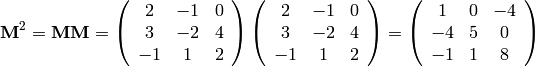
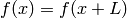
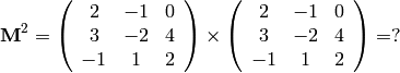
If
What is 
i.e., what is the matrix matrix product?
Go that one? Good.
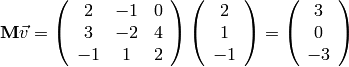
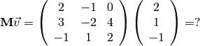
What about this matrix vector product?
We will use a single-column matrix for the vector  is
is

What is  ?
?
(Also, we will usually leave the symbol out)
Check your answers here before going on.
11.2.2. A Linear System of Equations
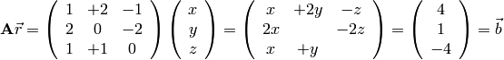
Here’s a typical linear algebra problem. Let’s say you need to solve
these three coupled linear equations for the variables  , and
, and  .
.
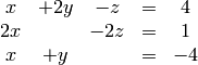
These are linear equations because the variables , and appear in linear form,
i.e. raised to the 1st power,  , as opposed to quadratic
  ,
cubic
,
cubic  , or other non-linear (
 ) powers.
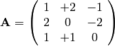
You could also write this in matrix form.
Let

and

Remembering the rules of matrix vector multiplication.
We can write our three linear equations very succinctly as  .
.
where  is the matrix on the left,
  is the
(column-matrix) vector of unknowns [
is the
(column-matrix) vector of unknowns [  ], and
 is the vector on the right side.
Let’s now define another (unknown) matrix:  which will be the inverse of A.
If was a normal scalar variable (like 5, or  ), let’s call it
  ,
then the inverse of would be
,
then the inverse of would be  . Then
For matrices, given , we want to find another matrix
, defined such that if you multiply  you get something like
  (One).
In matrix algebra, (One) is called The Identity Matrix. It is the matrix
that you can multiply times ANY matrix  , and get the same matrix as the
result.
, and get the same matrix as the
result.
That’s what  (One) does for scalar numbers: for any ,
  .
.
The Identity Matrix,  , looks like this (in 3-dimensions):
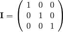
Try it yourself:
Multiply
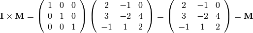
Please check that this is true.
The Inverse of matrix is another matrix, which we write as ,
such that if you multiply you get , the Identity matrix.

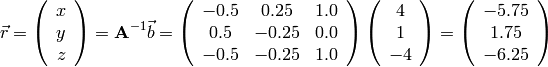
Now, if we knew the inverse, , of ,
we could use this to find the vector of unknowns in our original problem—the linear set of equatoins
we started with.
Because, if
then, multiply both sides of the equation above,  , by
, by
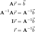
Wow! All we have to do is find the matrix and we can use it to find our unknown vector
 , and solve the set of linear equations. The solution is just

On to Octave.
11.2.3. A Taste of Octave
We will use a free “clone” of Matlab, called Octave. It doesn’t have all the fanciest features of Matlab–it actually uses Gnuplot for its graphics, but it does have much of the numerical linear algrebra capability. Octave comes standard on Fedora Scientific., so you can run it on your own computer; you don’t have to log on to another computer.
To start Octave, simply open a terminal and type:
octave.
You should see this:
GNU Octave, version 3.0.3
Copyright (C) 2008 John W. Eaton and others.
This is free software; see the source code for copying conditions.
...

octave:1>
Once again, you get a prompt:
octave:1>
waiting for input.
At the octave:1> prompt, type:
octave:1> A = [1, 2, -1; 2, 0, -2; 1, 1, 0]
When you hit ENTER, octave responds with
A =

   1   2  -1
   2   0  -2
   1   1   0
You have just entered the *matrix form of .
Notice the octave syntax for matrices:
- elements in a row are separated by commas [1 , 2 , -1; 2 , 0...]
- rows are separated by semicolons; [1, 2, -1 ; 2, 0, -2 ; 1, 1, 0]
Next enter the  vector. is a single-column matrix, with
only one element per row, so each entry is separated by a semicolon “;“
vector. is a single-column matrix, with
only one element per row, so each entry is separated by a semicolon “;“
octave:2> b = [4; 1; -4]
b =

   4
   1
  -4
Now, to find , the *inverse of , type
octave:3> Ainv = inv(A)
Ainv =

  -0.50000   0.25000   1.00000
   0.50000  -0.25000  -0.00000
  -0.50000  -0.25000   1.00000
We have defined a new matrix named Ainv and called octave’s matrix inverse function: inv().
Octave uses the star * for matrix multiplication.
Let’s check that  .
.
Mathematically, we are asking if
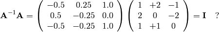
You can check this “by hand”, or use Octave.
At the octave:> prompt type
octave:4> Ainv * A
ans =

   1   0   0
   0   1   0
   0   0   1
We have shown that indeed, Ainv = .
Now let’s solve those coupled linear equations. Type:
octave:5> Ainv * b
ans =

  -5.7500
   1.7500
  -6.2500
There you go:
The unknowns, , and are
In other words, the solution of the original set of equations is
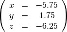
Pretty easy. You can verify that these solve the above equations.
Consider the last equation of the set:

Indeed:  .
.
Probably this doesn’t seem like we did rocket science, but imagine if we had a system of 500 coupled linear equations! It would be just as easy, except for typing in the matrix and vector, which you probably would program Octave to construct the vector for you.
At least now, you have a little taste of what Octave can do.