11.1. Symbolic Math and Numerical Linear Algebra
Now that you know how to logon to the Physics department’s utility computer, physics-nix.stk.pacific.edu, you can use some of its specialized software. Actually this machine is VERY old! There is a new replacement for it sitting in a box beside it, but that will have to wait for time later in the summer to install. Nonetheless, you can get started using the old machine. So far, we’ve learned about
- The Scientific Environment
- Unix
- Gnuplot
- Latex
- Xfig
- SSH/SFTP
The only time we got to do anything like real science was using gnuplot where we plotted some data, did some fits, and made a prediction about the population.
Let’s return to tools for doing science and math.
11.1.1. Doing Symbolic Calculations (algebra and calculus) with Mathematica
Much of scientific computing is about manipulating numbers: computing them, graphing them, interpreting them , etc. But math is the language of science, and so it would be nice if we can also use the computer to do math.
Of course we can do math—and have. In our Gnuplot investigations we solved
the equation 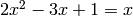 , graphically . This however
involved a numerical method, successively limiting the x range to
find where the left and right sides were equal. The solution was good
to about 6 decimal places (since that’s the limit of our x-range
accuracy in those plots).
, graphically . This however
involved a numerical method, successively limiting the x range to
find where the left and right sides were equal. The solution was good
to about 6 decimal places (since that’s the limit of our x-range
accuracy in those plots).
Also using Gnuplot, we can plot interesting mathematical functions,
such as the ArcTangent  and the Bessel function
  . However, what
gnuplot does is generate tables of numbers to plot for these
functions.
. However, what
gnuplot does is generate tables of numbers to plot for these
functions.
We can’t really do algebra, calculus, or differential
equations with gnuplot—these require Symbolic Math Calculations, the
manipulation of abstract variables, a, b, g and operations like  .
For this we use tools like
.
For this we use tools like
- Mathematica (Wolfram Inc.)
- Maple (Maplesoft Inc.)
Another tool you may have used or heard about is: Matlab. Matlab is a numerical linear algebra tool. We’ll talk about it in the next section.
The two above are the leading packages (as of now) of the tools for symbolic math on the computer, and as you can see they are commercial applications meaning they are not free. An enormous amount of research and work has gone into creating software environments that can do math the way you do it in math class: manipulating variables according to the rules of algebra, trigonometry, calculus, differential geometry, combinatorics, etc. Thus these packages are not cheap: both Mathematica and Maple sell at about $1000 for the basic package (however there are student versions for each at $100-150.
While my philosophy is strongly geared toward providing you with Free software, there is nothing in the Free realm that compares to these systems. There is an open-source Python project called Sage, which is being developed. But it is not as powerful as these other tools (yet).
We can, however, give you access to some of these commercial tools because the university has site licenses and these packages are available on certain machines. For the moment, we will explore Mathematica. This was part of the purpose of teaching you to login on remote machines. Now the university (and you!) can save money by putting special software on certain machines and then giving students and faculty access to those machines. This is one of the purposes of our machine: physics-nix.stk.pacific.edu.
11.1.1.1. Let’s play with Mathematica
We won’t be able to delve deeply into using Mathematica–for that Wolfram Inc. offers courses, online seminars, trainers and consultants. However, once I give you access to Mathematica, one of the easiest ways for you to get deeper into it is to Google “Mathematica Tutorial” or “Introduction to Mathematica” and look at the many (excellent) things that exist on the Web.
My purpose here is to just wet your appetite by showing you how to get started, how to do a couple basic things, and then give you pointers to more documentation.
First, you need to be logged onto physics-nix.stk.pacific.edu as user phystu. You remember how to do that, right? .
At the prompt, type:
phystu@physics-nix[~]> math
You should get the following response:
Mathematica 7.0 for Linux x86 (32-bit)
Copyright 1988-2009 Wolfram Research, Inc.

In[1]:=
The Mathematica prompt is In[1]:= and this indicates that it is waiting for input.
If you DO NOT get this response, but instead get :
phystu@physics-nix[~]>math
Mathematica 9.0 for Linux x86 (32-bit)
Copyright 1988-2012 Wolfram Research, Inc.

/home/phystu/.Mathematica/Licensing/mathpass:2:
        The Mathematica license you are using has expired.
        Please contact Wolfram Research or an authorized
        Mathematica distributor to extend your license and
        obtain a new password.

/home/phystu/.Mathematica/Licensing/mathpass:3:
        The Mathematica license you are using has expired.
        Please contact Wolfram Research or an authorized
        Mathematica distributor to extend your license and
        obtain a new password.

/home/phystu/.Mathematica/Licensing/mathpass:4:
password file "/home/phystu/.Mathematica/Licensing/mathpass".
        Invalid password.

/home/phystu/.Mathematica/Licensing/mathpass:5:
password file "/home/phystu/.Mathematica/Licensing/mathpass".
        Invalid password.

Mathematica cannot find a valid password.

For automatic Web Activation enter your activation key
(enter return to skip Web Activation):
Just type CTRL-d to exit.
This indicates that someone else is using Mathematica on physics- nix at the moment.
I’ve been trying to save money by just using a 2-seat licencse for Mma.
If you get this response, logout by hitting CTRL-d , wait some time, log back in, and see if your colleague has finished using Mathematica
If you are still having trouble getting a free session, email me and I’ll set up a schedule.
If you run into different problems, email me as usual.
Mma is a common abreviation for Mathematic and I will use it below.
Let’s assume now you have the Mma prompt, In[1]:=, waiting for you to tell it something.
Try the simplest thing: type 1+1 ENTER
In[1]:= 1+1

Out[1]=  2

In[2]:=
Mma responds to your input, by computing the sum of 1+1. Bet you knew that one...
11.1.1.1.1. Derivatives
Let’s try something more interesting. Most of you will have completed Differential Calculus (MATH 051 at Pacific).
I opened my freshman Calculus book and pulled out one of the problems I was assigned. Compute the following derivative:
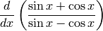
In Mma we would use the Derivative operation: D[...] like this. At the Mma prompt, In[2]:= (it might have another number than 2 on your computer).
In[2]:= D[(Sin[x] + Cos[x])/(Sin[x] - Cos[x]), x]
Then type, ENTER.
Mma responds with:
                                            2
        Cos[x] - Sin[x]    (Cos[x] + Sin[x])
Out[2]= ---------------- - -------------------
        -Cos[x] + Sin[x]                     2
                           (-Cos[x] + Sin[x])
In the In[2]:= command, do you see that the D (Derivative) operator acts on the function
(Sin[x]+Cos[x])/(Sin[x]-Cos[x]),
and takes the derivative with respect to x, which is the last argument to D[..., x]?
Let’s look closer at the Mma syntax.
Mma functions, operators, etc. (almost) ALWAYS begin with Capital letters: D**[...], **Sin[x], Cos[Pi x/2], and so forth.
Arguments to functions and operators are enclosed in square brackets: Sin[x**]**, Exp[x^2/a ], and so on.
This is special to Mma. Gnuplot, and most programming languages, by contrast, use lower case functions with parentheses like this: sin(x). So, it can sometimes be confusing when switching back and forth between programs.
Just be aware: Mma uses CAPS and []’s
The answer given in Out[2]= is correct. Mma has applied the Chain Rule with the appropriate Trig derivatives, but it’s not the simplest form for the result. For this, there is a handy function: Simplify[]
In[3]:= Simplify[%]

              2
Out[3]= -------------
        -1 + Sin[2 x]
Notice that I used the % (percent) here. The % symbol in Mma means “the result of the last command”.
Note that sometimes the Simplify command helps and sometimes not. But it’s worth a try.
11.1.1.1.2. Solving (non-linear) Equations
Let’s see what Mma does with the equation we solved using gnuplot:
.
For this we use Mma‘s Solve[] function. We have to give it the equation we wish to solve.
Mma‘s syntax for an equation is:
2x^2 - 3x + 1 == x
Notice I’ve used the ^ (caret) to mean exponentiation of a power.
Also, the == in the above statement indicates a relation of equality between two things. This is how we tell Mma that the thing above is an equation, as opposed to an assignment.
If we wrote 2x^2 -3x + 1 = x, with = instead of ==, we would be telling Mma to assign x (the RHS) to 2x^2 -3x +1 (the LHS), in the same way you assign a variable y the value 5, by typing y = 5.
Next we pass this equation to the Solve[] function, and tell it to solve the equation for the variable x.
In[7]:= Solve[2x^2 - 3x + 1 == x, x]

               2 - Sqrt[2]         2 + Sqrt[2]
Out[7]= {{x -> -----------}, {x -> -----------}}
                    2                   2
Very good. This is a quadratic equation, there are two solutions, and there they are. You can check by hand if you like.
11.1.1.1.3. Root Finding
How about another more interesting equation,
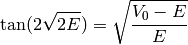
say, the one from the end of Homework 5:
using  ?
?
If we just plug it into the above syntax, we get this:
In[8]:= Solve[Tan[2Sqrt[2E]]==Sqrt[(50-E)/E], E]

General::ivar: E is not a valid variable.

Out[8]= Solve[False, E]
Oops! In Mma, E is a protected character (like Pi).
It’s Euler’s number:  .
.
Try this: Use x for E in the above equation:
In[9]:= Solve[Tan[2Sqrt[2x]]==Sqrt[(50-x)/x], x]

Solve::tdep: The equations appear to involve transcendental functions of the
    variables in an essentially non-algebraic way.
Still... no joy. But definately an interesting reply from Mma.
Mma is saying that this equation is transcendental and can’t be solved in closed (algebraic or symbolic) form . Still we can ask it to Numerically solve the equation–that is, put numbers in the equation for x, and change x until we get a numerical answer that satisfies the equation to the accuracy we need. As long as there is only one variable, x, this will work.
We do this with the function: FindRoot[ eqn, {var, starting_guess } ]
Recall that a Root of an expression is an x value where the expression = 0. However Mma is
smart enough to know that the x value that solves 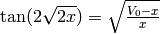 is a Root of the expression:
 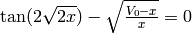 .
.
We have to give Mma a little help with an initial guess. Let’s start at x = 0.
In[12]:= FindRoot[Tan[2Sqrt[2x]]==Sqrt[(50-x)/x], {x,0}]

                                 1
Power::infy: Infinite expression -- encountered.
                                 0.
Duh. Should have seen that coming. The RHS is infinite at x=0. So, start with a small positive guess: 0.00001
In[13]:= FindRoot[Tan[2Sqrt[2x]]==Sqrt[(50-x)/x], {x,0.00001}]

Out[13]= {x ->  0.279726}
Booyah!
This should be close to what you got using the graphical method (zero-ing in on the place where the two sides are equal) with Gnuplot. My solutions using gnuplot are shown here.
The other solutions from Mma are:
In[15]:= FindRoot[Tan[2Sqrt[2x]]==Sqrt[(50-x)/x], {x,0.5}]
Out[15]= {x ->  2.5157}
In[17]:= FindRoot[Tan[2Sqrt[2x]]==Sqrt[(50-x)/x], {x,3}]
Out[17]= {x ->  6.97724}
In[19]:= FindRoot[Tan[2Sqrt[2x]]==Sqrt[(50-x)/x], {x,8}]
Out[19]= {x ->  13.6399}
In[22]:= FindRoot[Tan[2Sqrt[2x]]==Sqrt[(50-x)/x], {x,20}]
Out[22]= {x ->  22.4543}
In[23]:= FindRoot[Tan[2Sqrt[2x]]==Sqrt[(50-x)/x], {x,30}]
Out[23]= {x ->  33.309}
In[24]:= FindRoot[Tan[2Sqrt[2x]]==Sqrt[(50-x)/x], {x,45}]
Out[24]= {x ->  45.8083}
We get these by giving starting points near the expected answer, and we can find those expected answers by using Gnuplot to look at graphs of the functions.
Compare the Mma results above with my graphical solutions from HW 5.:
# State   Energy
 1         0.280
 2         2.502
 3         6.976
 4        13.643
 5        22.455
 6        33.307
 7        45.811
11.1.1.1.4. Integration
Before we leave Mma, let’s do some integrals!
Start with the simplest one: 
In[1]:= Integrate[x,x]

         2
        x
Out[1]= --
        2
Nice. It’s good to know things you learned in grade school are still true.
The syntax of the Integrate function in Mma is:
- Indefinate integrals: Integrate[ integrand , variable ] or
- Definate integrals: Integrate[ integrand , { variable , lowerLimit, upperLimit}]
In the first case, like the trivial case above, we did an indefinate integral which returns a function (the anti-derivative).
The second version of the Integrate[] function is for a definate integral, when the integral has a lower and an upper bound, and the answer is a number.
Indefinate Integrals
Here’s a more interesting integral:
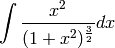
This one is a little more complicated, and I bet you don’t know the answer by looking at it.
Mma gives:
In[8]:= Integrate[x^2/(1 + x^2)^(3/2), x]

               x
Out[8]= -(------------) + ArcSinh[x]
                    2
          Sqrt[1 + x ]
Now, that would have taken a little work on paper..
Definate Integrals
On to Definate Integrals.
What is this one: 
In[2]:= Integrate[x, {x, 0, 1}]

        1
Out[2]= -
        2
OK, let’s be serious. Here’s another one from my freshman calc book:
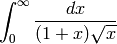
We code this in Mma as follows:
In[4]:= Integrate[1/((1+x)Sqrt[x]), {x, 0, Infinity}]

Out[4]= Pi
Notice a couple things here:
Unlike Gnuplot, where we MUST explicitly put the * operator in for multiplication, as in x*y, Mma understands our usual algebraic expression: xy or x y (with just a space) as x “times” y.
Notice that the Mma code, with the extra ()’s
1/((1+x)Sqrt[x])
as we typed above, would be very different from this
1/(1+x)Sqrt[x].
without the extra ()’s.
The first version evaluates to
![{\tt 1/} {\bf (} {\tt (1+x)Sqrt[x]} {\bf )} ~~~~\Rightarrow ~~~~ \frac{1}{(1 + x)\sqrt{x}}](../_images/math/0caad10ed3d7db4f0299beb8b770548b74583d96.png)
while the second, without the extra set of ()’s would be:
![{\tt 1/(1+x)Sqrt[x]} ~~~~\Rightarrow ~~~~ \frac{1}{(1 + x)}\sqrt{x}](../_images/math/8db18b041bf7efc6df697ffad8c5a9f26f451546.png)
Warning
Make sure you understand this suble difference!
Also, notice that we used one of the built in Mma constants above: Infintity. Mma also understands (Capital) Pi, as shown below.
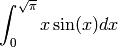
In[6]:= Integrate[ x Sin[x^2], {x, 0, Sqrt[Pi]}]

Out[6]= 1
I think you are getting the picture.
Have a look at this document
Then, if you want to learn more look at:
- Mathematica Tutorials at Wolfram.com
Also, a very nice, free website is Wolfram Inc.’s Integrals.
Check it out! Now that you know Mma syntax for functions (Sin[], etc.), you enter almost any function whose integral is known, and this site will return the answer to you.
That could come in handy, eh?
This gives you a taste of symbolic math on computers. I would love to go further and show you, for example, the Mma packages for doing Riemann Tensor Calculus in General Relativity, but your head would explode. Hopefully, this taste of Mma will get you started, at least enough for your freshman physics and math needs.