6.2. Fitting Functions to Data
So, now we can do science, i.e. discover something about the world.
We’ll start with a trivial example.
Suppose you and a friend are confronted with the following circuit in lab (likely you did this in the 5rd grade, or later in PHYS 55).
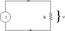
You have a variable (i.e. at your control) current source, I, in a simple circuit with a resistor, R, whose value you do not know.
As your friend varies the current, you are able to measure the voltage, V, across the resistor. As you know from your studies of circuits, the voltage should be related to the current by Ohm’s Law:
V = IR
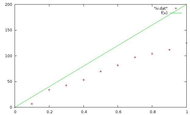
Thus, if you plot your measurements of V versus I, you could find the resistance, R, from the slope of the line that goes through your data.
Here’s the data. You can also download the file iv.dat to save you typing it in by hand (right-click, Save Link).
# I    V_R
#amps volts

0.00  0.00
0.10  6.77
0.20  33.84
0.30  42.38
0.40  53.07
0.50  69.87
0.60  81.45
0.70  96.91
0.80  103.90
0.90  111.99
1.00  125.11
Before we begin, notice that the data file has comments at the top, lines which begin with a ‘#’ . You can put comments anywhere in your data file; everything on the line after a ‘#’ will be ignored by gnuplot.
Start gnuplot and plot this data.
You can see that the voltage rises sort of linearly with increasing current.
Estimate the slope by eye.
What is your estimate? (write it down or remember it for later)
Let’s try to fit a line to the data “by hand”.
Define a linear function: B
f(x) = a*x + b
(that’s a line, right?)
Since the first data point is (0,0), and since Ohm’s law has no constant term, let’s set:
gnuplot> b = 0
(Knowing this, we could just as easily defined f(x) = a*x.
To set a, take your in initial guess from above:
gnuplot> a = your estimate from above
This is a number! You will be typing something like ‘a = 200’.
Now, plot the data and your function together.
gnuplot> plot "iv.dat", f(x)
How well does your guess match?
You can refine your guess by typing a new value for a, and doing ‘replot’. If the ‘f(x)’ line is too steep, set a lower.
Try it.
Do you see how the line changes as you change the slope, a? Try to zero in on the best line that “fits” your data.
What is your best estimate of a?
6.2.1. Least Squares Fit
Gnuplot has a wonderful builtin command to automate this process, in a very powerful and flexible way.
The command is called, not surprizingly, ‘fit’. You use it like this:
gnuplot> fit f(x) "iv.dat" via a
gnuplot> plot "iv.dat", f(x)
The syntax of the ‘fit’ command is:
‘gnuplot> fit function “datafile” via var1, va2, var3,...’
Here
- fit is the fitting command (this is always the same).
- function is a function which you have defined, including some “variables” within it, such as ‘f(x) = a3*(x**3) + a2*(x**2) + a1*x + a0’.
- “datafile” is the file where your data is located. Remember that since this is a file , you must refer to it enclosed in “”s.
- via var1, var2, var3,... are the parameters (the constants) you want gnuplot to tweak until it gets the best fit. You must have at least one parameter var1, and the keyword via.
When you run the ‘fit’ command, it will spew a fair amount of information as it changes each of the variables you specified after ‘via’.
Finally, it will converge on the ” Best ” values, and print a summary of the results, which looks like this:
gnuplot> fit f(x) "iv.dat" via a
...

After 3 iterations the fit converged.
final sum of squares of residuals : 231.793
rel. change during last iteration : -8.79516e-08

degrees of freedom    (FIT_NDF)                        : 10
rms of residuals      (FIT_STDFIT) = sqrt(WSSR/ndf)    : 4.81449
variance of residuals (reduced chisquare) = WSSR/ndf   : 23.1793

Final set of parameters            Asymptotic Standard Error
=======================            ==========================

a               = 130.403          +/- 2.454        (1.882%)


correlation matrix of the fit parameters:

               a
a               1.000
This contains some statistical information about your data and the level of its randomness, most of which is beyond the scope of this course. However, it’s nice to know that it’s there as you learn more about statistics in subsequent courses. We’ll look at these things a little bit soon.
The important line is:
Final set of parameters            Asymptotic Standard Error
=======================            ==========================

a               = 130.403          +/- 2.454        (1.882%)
This is your result: you have just analyzed your data and found the resistance, R, to be about 130 Ohms, plus or minus 2.5 Ohms.
Whoa...